The Latency Lie: Why Your Control Loop Is Slower Than Your Spec Sheet Claims

A controls engineer's field guide to the hidden microseconds that destroy precision

June 22, 2026 · RobustMotion

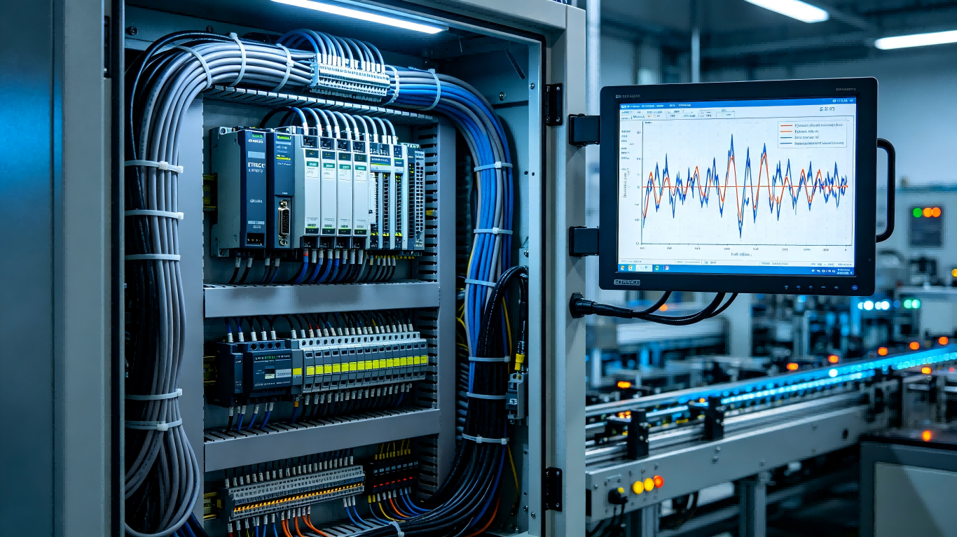
You read the datasheet. 1 kHz servo update rate. EtherCAT cycle time: 250 microseconds. The vendor's application note shows a pristine step response: command, response, settling. No overshoot. Perfect tracking. You sign the purchase order confident that your control bandwidth is sufficient for the application.

Then you commission the line. The gripper approaches the workpiece at 50 mm/s. Contact. Force spike. Cracked substrate. Scrapped part. Root cause analysis points to 'excessive approach velocity.' You slow to 10 mm/s. Same result. You slow to 2 mm/s. The process works, but your cycle time is now unacceptable. The quality team approves, but operations puts the cell on a watch list. And somewhere in the back of your mind, a question forms that the datasheet never answered: where did the microseconds go?

The answer is that they were never there to begin with. Not as usable control bandwidth. The 1 kHz update rate is a theoretical maximum under ideal conditions. The real-time performance of your distributed control architecture is determined by the slowest, dirtiest, least deterministic segment of the signal chain. And in most precision automation cells, that segment is the cable run between the drive cabinet and the actuator endpoint.

The Stack of Delay

Consider the complete signal path for a force-controlled gripper in a typical architecture. The force sensor analog signal is digitized by a conditioning module. The digital value traverses a sensor cable to the gripper junction box. From there, it travels via a fieldbus segment to the I/O module. The PLC reads the input, executes the force control algorithm in its cyclic task, computes a motor torque command. The command is written to an output register, transmitted across the fieldbus to the servo drive. The drive's position loop interpolates, the velocity loop calculates, the current loop modulates. The PWM signal reaches the motor. The motor produces torque. The torque moves the mechanism. The mechanism contacts the workpiece.

Each arrow in this chain represents latency. Some are deterministic and documented. Many are not. The sensor conditioning module's internal filter. The fieldbus junction box's store-and-forward buffer. The PLC task scheduler's jitter when the HMI update coincides with the motion task. The servo drive's interpolation delay when the command arrives mid-cycle. The current loop's PWM update phase.

Individually, each delay is microseconds. Collectively, they accumulate to milliseconds. And in force control at contact, milliseconds are geological epochs.

The vendor's 1 kHz specification assumes a direct connection between drive and motor, with the control algorithm executing in the drive's own processor. It does not account for the architectural reality of your cell: a PLC running the application logic, a fieldbus mediating the conversation, and a control loop that closes across three physical devices and two communication protocols.

The Contact Event

The physics of mechanical contact is unforgiving. When a gripper finger traveling at 50 mm/s encounters a rigid surface, the force rise time is determined by the approach velocity and the combined stiffness of the contact pair. For typical metal-on-ceramic contact, the force can reach destructive levels in 2-3 milliseconds.

A control loop with 1 millisecond effective latency has one, perhaps two, control cycles to respond. But the loop latency is not the only constraint. The mechanical system itself stores energy. The motor rotor has inertia. The gearbox has backlash. The finger structure has compliance. When the controller finally commands deceleration, these stored energies release into the contact, producing the overshoot that the control algorithm never saw coming.

The result is a familiar commissioning pattern: slower approach velocities reduce the impact energy, extending the force rise time, giving the control loop more cycles to respond. But slower approaches directly consume cycle time. The cell becomes a bottleneck. Operations demands a solution. Engineering proposes mechanical compliance—springs, elastomer pads, flexure joints—to absorb impact energy. The compliance works, but it introduces positional uncertainty. The process window narrows. The quality team adds inspection steps. The line that was designed for speed now crawls through its sequence, buffered by WIP, monitored by engineers, and tolerated rather than trusted.

The Integration Alternative

The architectural alternative is not faster buses or more powerful PLCs. It is the elimination of the architectural separation that creates the latency stack.

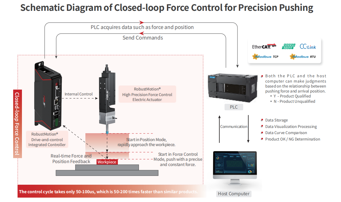
Drive-and-control integration places the servo amplifier, the motion processor, and the sensor interfaces within a single module, typically co-located with the actuator. The force sensor signal reaches the control algorithm without traversing a fieldbus. The motor current command is computed and issued in the same processor cycle. The loop frequency is limited by the processor's interrupt capability, not by the propagation delay of a communication protocol.

Frequencies of 10 kHz—ten thousand control cycles per second—become practical. At this rate, the control loop executes every 100 microseconds. The force rise time of a contact event, measured in milliseconds, now spans tens of control cycles. The controller has time to observe, predict, and respond. Not merely react after the fact, but anticipate contact based on position and velocity trajectory, modulating motor torque before the force sensor registers impact.

This is not incremental improvement. It is a qualitative change in what the control system can know and when it can act. The difference between 1 kHz and 10 kHz is not a factor of ten in performance. It is the difference between a system that can control force and a system that can only limit damage.

The Unified Control Problem

The deeper advantage of integration emerges when the control task is not merely fast, but unified. In a distributed architecture, position control and force control are typically implemented in different devices with different clock domains. The position loop runs in the servo drive. The force loop runs in the PLC. The handoff between them is a protocol transaction, a mode switch, a state transition that takes time and introduces transient behavior.

In an integrated module, both algorithms execute on the same processor, accessing the same sensor data, sharing the same clock. The transition from position mode to force mode is a branch within a single control task. Both variables can be regulated simultaneously, with dynamically weighted priorities that shift based on process state. During approach, position dominates. At contact, force takes precedence. During insertion, a hybrid blend maintains both constraints.

This unified control enables strategies that are impractical in distributed architectures. Impedance control, where the actuator presents a programmable mechanical stiffness to the environment. Admittance control, where the actuator follows external forces with programmable compliance. Predictive force limiting, where the controller models the mechanical system and pre-computes the torque trajectory that achieves desired contact dynamics without overshoot.

These are not theoretical constructs. They are the control foundations of precision assembly processes that cannot tolerate destructive contact: semiconductor die handling, medical device assembly, optical component placement, battery cell stacking. Processes where the cost of a single scrapped workpiece exceeds the cost of the entire actuator.

The Specification Problem

For the engineer evaluating motion control options, the challenge is that traditional specifications obscure the architectural reality. The datasheet reports servo update rates, bus cycle times, and positioning accuracy under static conditions. It does not report effective control loop latency under distributed operation. It does not report force overshoot at contact. It does not report the commissioning time required to achieve stable force control across product variants.

The result is a specification mismatch: systems are selected based on metrics that don't predict real-world performance, then deployed in architectures that compromise the very performance they were selected for. The 1 kHz drive is purchased for a 10 kHz problem. The precision actuator is connected through a non-deterministic bus. The force sensor is digitized by a module with a 5 ms filter constant. Each decision is individually reasonable. The system integration is collectively broken.

The Honest Architecture

The path forward requires architectural honesty: matching the physical distribution of control intelligence to the temporal and spatial demands of the application.

For large machines with separated axes, distributed architectures retain advantages. The drive cabinet is close to the motors. The control loops are local. The communication distances are short. The latency stack is manageable.

For end effectors, compact actuators, and precision assembly nodes, the opposite is true. The actuator is at the end of a cable run. The control loop traverses multiple devices. The latency stack dominates performance. The architecture that works for a five-axis CNC is precisely wrong for a force-controlled gripper.

The integrated module is not a compromise or a cost-cutting measure. It is the correct architecture for a class of control problems that distributed systems were never designed to solve. It recognizes that in precision automation, the most critical control loop is not the one that tracks position. It is the one that manages contact. And contact happens at the actuator, not in the cabinet.

For the engineer who has watched force traces ring with overshoot that no tuning could eliminate, who has slowed approach velocities until the cycle time became a line bottleneck, who has added mechanical compliance that introduced more problems than it solved—the integrated alternative offers something beyond technical performance. It offers architectural coherence. A system whose physical structure matches the control problem it is asked to solve.

The microseconds that disappeared in your distributed architecture were not lost. They were spent traversing cables, protocols, and clock domains that served no purpose in your actual control problem. Reclaiming them is not a matter of faster components. It is a matter of simpler topology. Control where the action is. Sense where the contact happens. Compute where the loop closes.

The latency lie is not a vendor conspiracy. It is an architectural inheritance from a time when motion was centralized and control was distant. Precision automation has outgrown that assumption. The question is whether your next specification will recognize it.